Simulating a multi-layered neuronal model
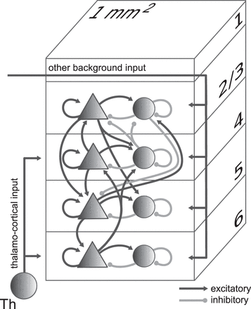
The mechanistic framework is based on the Dynamic Mean-Field model, a mathematical and computational framework used in neuroscience to study the dynamics of large-scale neural networks. It provides a simplified description of how the activity of neural populations can be modelled using the mean firing rate of the whole neuron population. We use the multi-layered model by Evers et al., as it adds cell-type specific connectivity to the balanced random network model developed by Van Vreeswijk et al. and Amit et al. Large-scale simulations of spiking neurons allow us to link structural information to neuronal activity. In the Dynamic Mean Field (DMF) model provided by Evers et al. 1, we first define the initial conditions of the system and the parameters, shown in Table 1 below as well as the connection probability and the structural connectivity of the local cortical layers Evers et al. shown in 1, where four out of the six layers (since 2 and 3 are combined) receive external thalamo-cortical input stimulation represented by the grey arrow. Each layer has both inhibitory (circles) and excitatory (triangles) populations of model neurons. The number of neurons in each population is extracted from 2. As for the connections, the excitatory (black) and inhibitory (grey) represent the connections between populations.

Figure 1: Model Definition. Extracted from Potjans et al. 3
Once all the general parameters have been established, we need to specify the simulation parameters. The simulation consists of three different parts. First, we have the pre-stimulation period of 0.5 seconds of no-input simulation. Then, we continuously stimulate a specific amplitude to two different neuronal populations for 2 seconds. Finally, there is the post-stimulation period, also known as the “baseline” where no external input is present. This last one extends for 10.5 seconds because the output of this simulation is later used to extract the BOLD signal, and the BOLD signal appears with a significant delay after the corresponding neuronal activity. Finally, we need to define the input current. We chose a range of stimulation input currents with intensities going from 50 to 300mA in 50mA jumps. Moreover, to the selected value from 4 the mentioned ranges, we add random uniform noise ranging from 50mA above and below that value to ensure we get the maximum uniformity in the input. These values are combined so that each simulation stimulates 2 out of the 8 populations, whether they are excitatory or inhibitory. The two intensities can also affect the same layer. So in the end we have an array with the layer combination as well as the input combination. It is important to keep the values since they are needed to train the neural net. The simulations were run in batches of 10 to reduce the computational burden. A baseline data set that included the simulation for those 10.5 seconds with no stimulus was saved. The baseline is independent of the simulation parameters because there is no current applied in this time interval. Therefore, an overall baseline array was saved and appended at the end of every simulation to optimize the code and reduce simulation time. We did all layer and input current combinations five times, for a total of 11520 simulations. As this was not enough data for the machine learning model, the process was repeated twice, for a total of 34560 simulations. The result for each simulation is the recorded intensity for each neuronal population. The appropriate function was extracted from Evers et al. 1. This variable, named Y, provides information about how the population’s activity changes in response to the experimental conditions, and it is the input for the next stage of this project.
| symbol | description | value |
|---|---|---|
| \( \sigma\) | noise amplitude | 0.02 |
| \( \tau_m \) | membrane time constant | 10e-3 |
| \( C_m \) | membrane capacitance | 250e-6 |
| \( R \) | membrane resistance | \( \frac{τ_m}{C_m} \) |
| \( g \) | inhibitory gain | -4 |
| \( M \) | number of populations | 8 |
| \( J_E \) | excitatory synaptic weight | 87.8e-3 |
| \( J_I \) | inhibitory synaptic weight | -35,12e-2 |
1: Kris S Evers, Judith Peters, and Mario Senden. “Layered Structure of Cortex Explains Reversal Dynamics in Bistable Perception”. In: bioRxiv (2023), pp. 2023–09.
2: Tom Binzegger, Rodney J Douglas, and Kevan AC Martin. “A quantitative map of the circuit of cat primary visual cortex”. In: Journal of Neuroscience 24.39 (2004), pp. 8441– 8453.
3: Tobias C Potjans and Markus Diesmann. “The cell-type specific cortical microcircuit: relating structure and activity in a full-scale spiking network model”. In: Cerebral cortex 24.3 (2014), pp. 785–806.